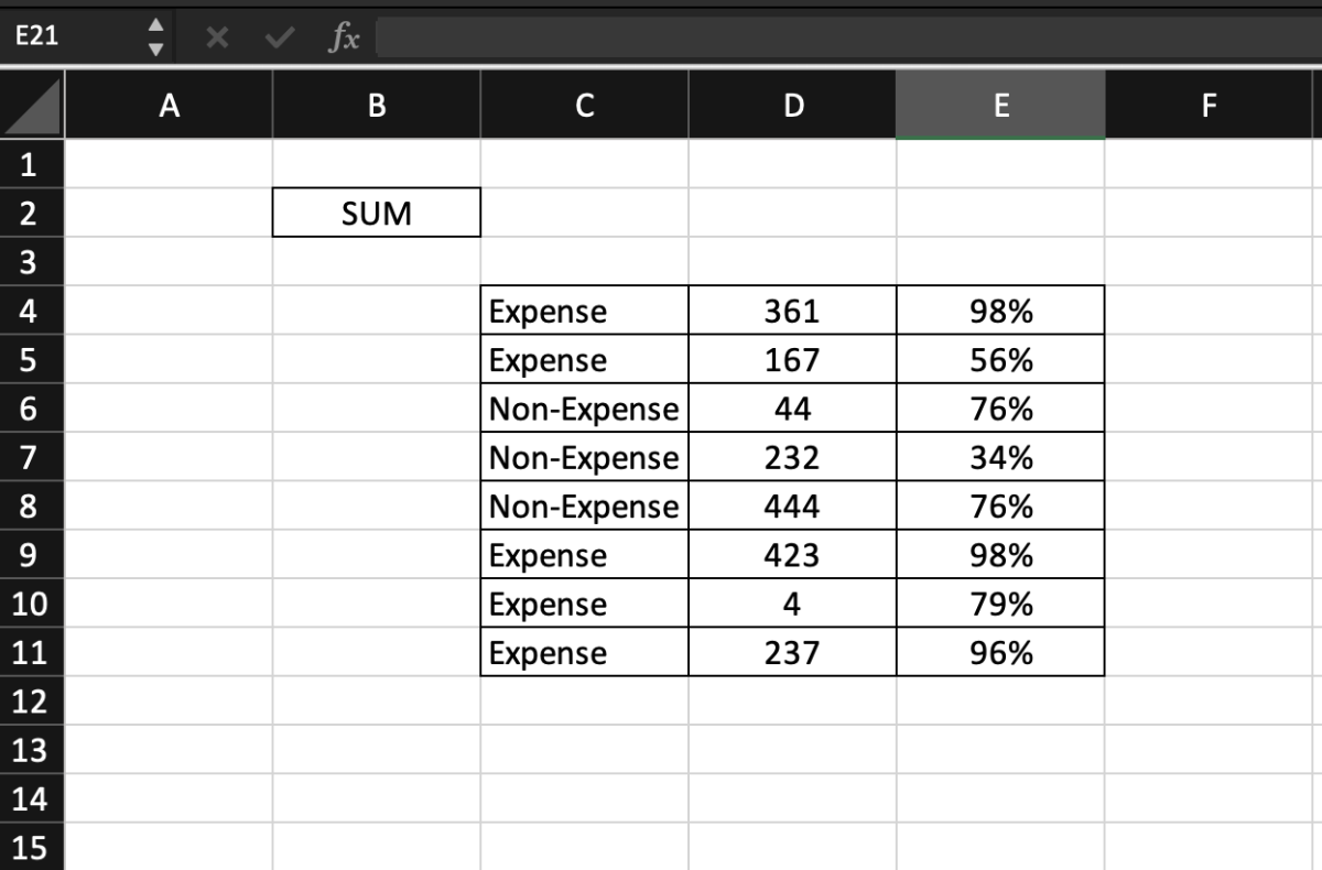
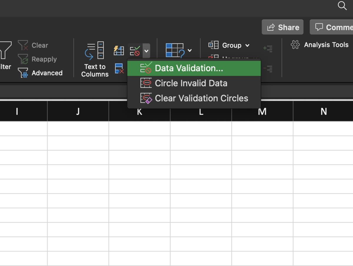
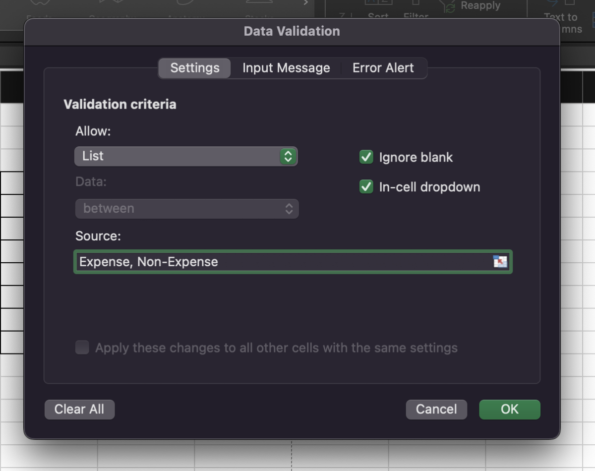
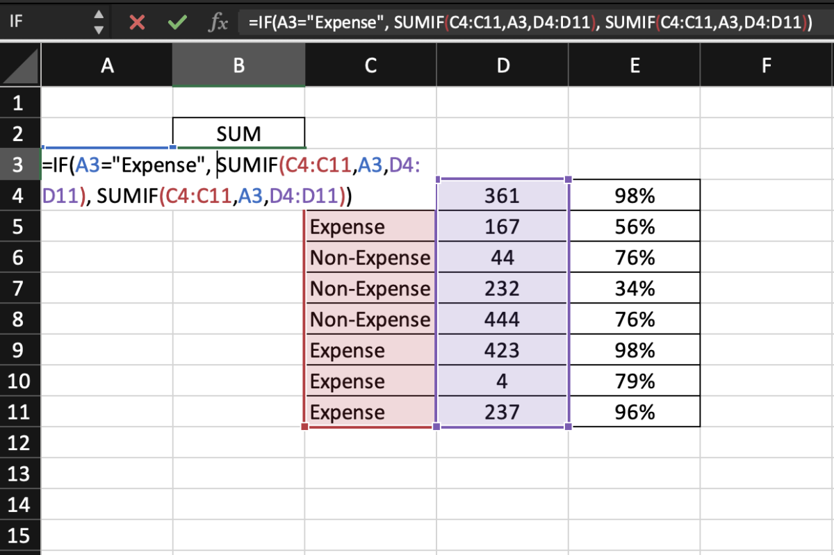
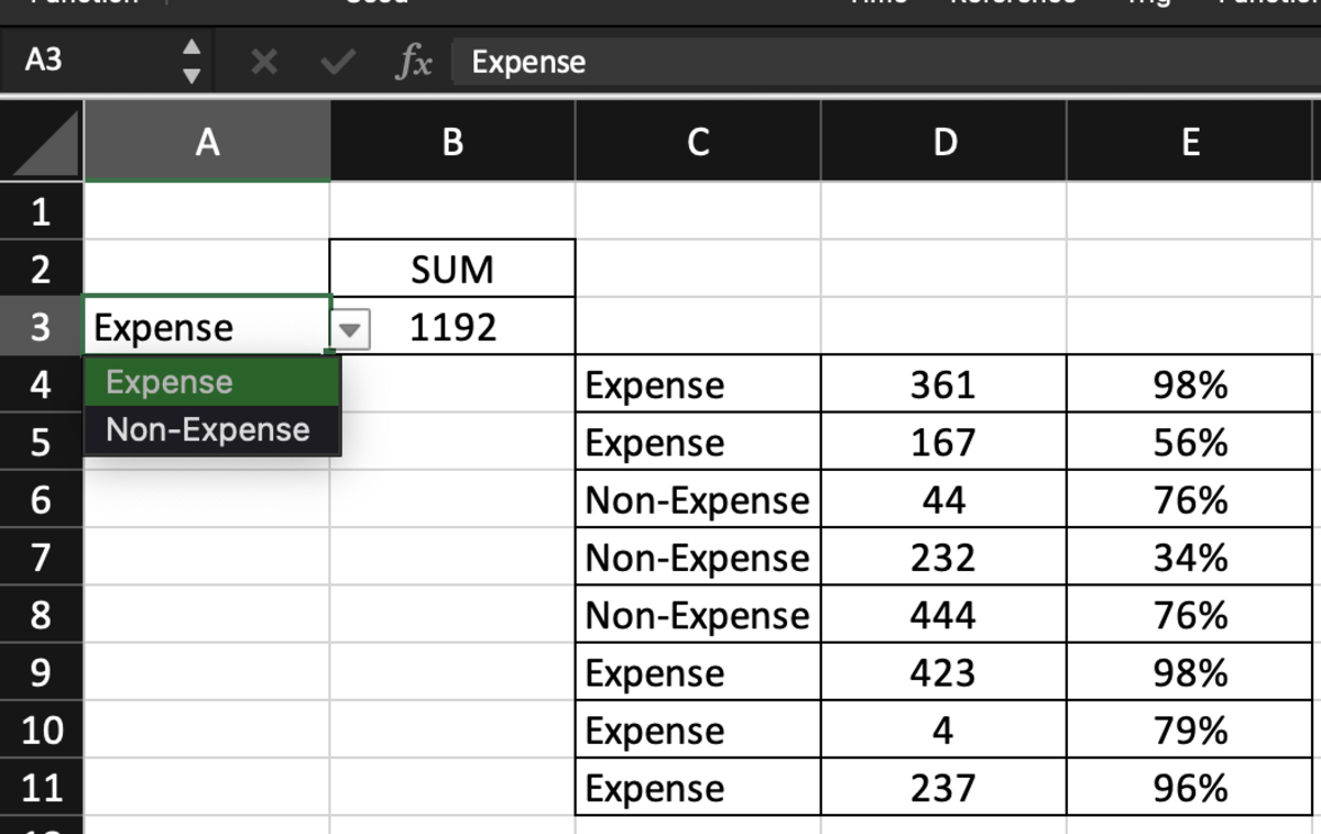
Below there is data categorized as expense and non-expense. My goal is to create a list box that will allow me to choose from “expense” and “non-expense” sums of the data set below. The list box will trigger the IF statement to make a decision and the SUMIF function will sum the data. First, I’m going to select the cell where I want the list box to appear. Next, I select the data tab and select the data validation option. I chose the list validation and entered the only two options that I want to appear in my list box. After selecting OK, the list box is active. I entered a lengthy equation that I will break down into segments. Look at the formula below. The if statement is dependent on the list box (expense/non-expense). If expense is chosen the first option will display. If not, the second option will display. I did repeat the formula, but you will see why when I go over the SUMIF part. List box Yes print this option No print this option =IF(A3=“Expense”, SUMIF(C4:C11,A3,D4:D11), SUMIF(C4:C11,A3,D4:D11)) In this part of the formula, I’m asking Excel to only sum D4:D11 for records that meet the same criteria as the list box. Meaning if expense is selected, only those records with values in column D will be added together. The duplicated formula is much like a placeholder for the IF function. It’s the same formula but will yield a different result when the list box value changes. SUMIF(C4:C11,A3,D4:D11)
Here you can see the options that can be toggled from the list box. This content is accurate and true to the best of the author’s knowledge and is not meant to substitute for formal and individualized advice from a qualified professional. © 2022 Joshua Crowder

